
|Ψ> = α|0> + β|1>
- Aug 29, 2021
- 4 min read
When learning any new programing language, lore has it that, one should start with the "Hello World!" script as a baseline and rite of passage into the community of developing code.
Today I am taking you on a journey through writing my first quantum program, the equivalent to "Hello Q-World!" which, in another timeline, would not be a big deal, but, unfortunately, I will not tolerate any such nonsense and adjust accordingly.
Getting down the workflow of writing an application and getting it to execute properly is the main goal of this lesson. Here is the link for the source code and video I am using for this blog.
There have been a few updates to Qiskit that render some of the commands from the video unusable with current versions, updated code will be provided when I get to the appropriate step.
Getting started is just as easy as it was in the post about installing Qiskit and the API token. Navigate into a Jupyter Notebook and we will begin.
from qiskit import *Using the wildcard as the import argument tells Qiskit it import all tools and libraries. Now comes building the quantum circuit.
In order to manipulate the qubits in our circuit, we need to build our quantum register. This is our variable that relates to the qubits that will be going into our circuit, and due to the nature of quantum mechanics, we also need to build a classical register to take measurements from the quantum bits. The code for this portion looks like this.
qr = QuantumRegister(2)
cr = ClassicalRegister(2)
We now have the ingredients to produce a two-qubit circuit.
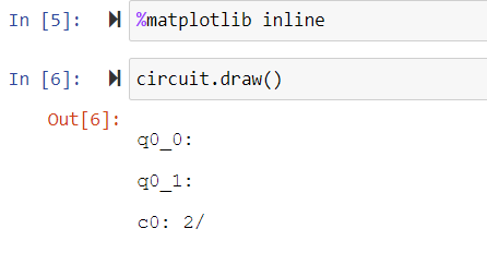
circuit = QuantumCircuit(qr, cr)Something neat that can be done, if at any point during your coding you'd like to visually see the circuit you can. Of the two pictures below, the first is how the code is executed currently as well as the code in the video.
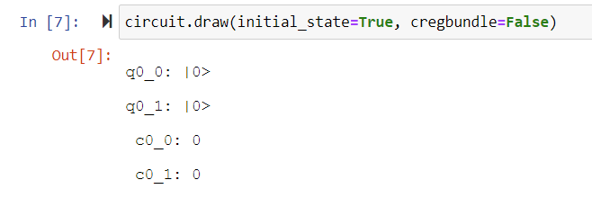
Below is the new command to elicit the same output as the video. By adding the code in the parentheses our notebook pumps out the "old" draw function, with updates to the platform things happen, and this was one of them.
There isn't anything really interesting happening with our circuit yet, lets add a Hadamard gate to our first qubit and see what happens? As I did, I can imagine you will need a primer on the Hadamard Gate, so, check it out here.
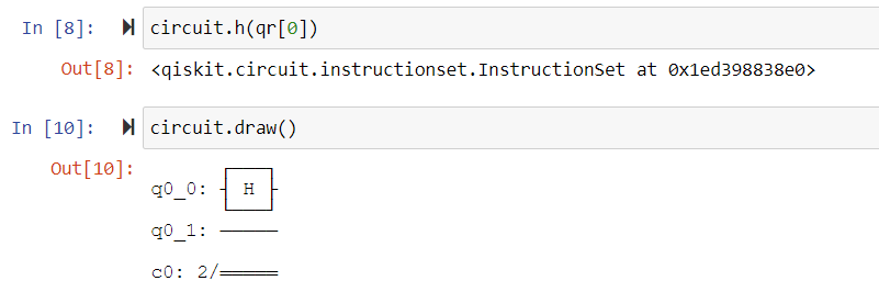
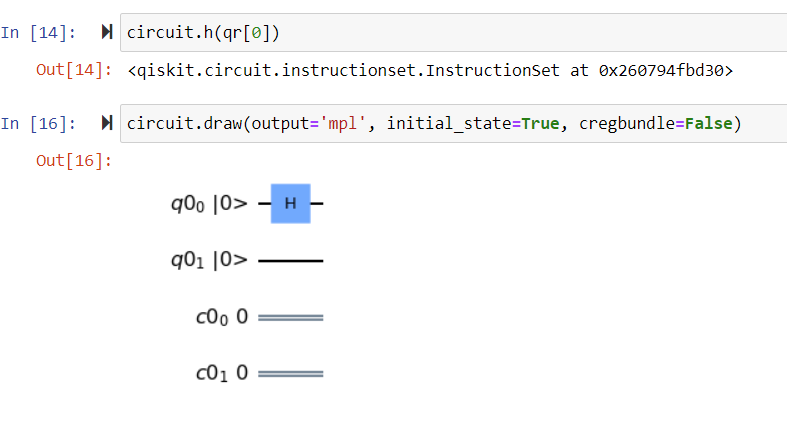
Now we can call our draw function again, however, instead of being a text-based output, we can have it presented graphically using:
circuit.draw(output = 'mpl')If we put all of the code together, we can produce a graphic of the circuit as seen in the video.
Not very much going on here so lets make things interesting by creating a 2 qubit operation, called a Controlled X, which is the quantum version of if this, then that. Here the first qubit will be targeting the second qubit, done like this.
circuit.cx(qr[0], qr[1])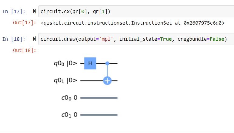
Our circuit now has a Hadamard Gate and a Controlled Not. With these two simple operations, we are able to generate entanglement between these two qubits that make up our circuit.
What we are going to do next is measure our quantum bits and store that measurement in our classical bits.
circuit.measure(qr, cr)Two things are going to happen next: first, I am going to run this program on my classical computer as a simulation of a quantum computer, secondly, I will then run the program on an actual quantum computer via my API token for IBMQ.
Aer is the quantum simulator that we will use for the classical simulation we will use to define our variable "simulator". The next block of code I will be posting will consolidate a few steps for the sake of time.
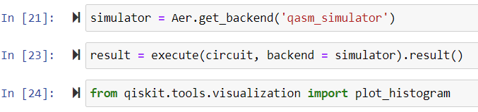
Line 23 is an all-in-one line. If you remove 'result =' and '.result()', you are left with just the execution of the circuit without keeping the results, so the additions are needed in order to gain data and insight into the circuit. Line 24 calls for tools within Qiskit for visualizing the output of the circuit.
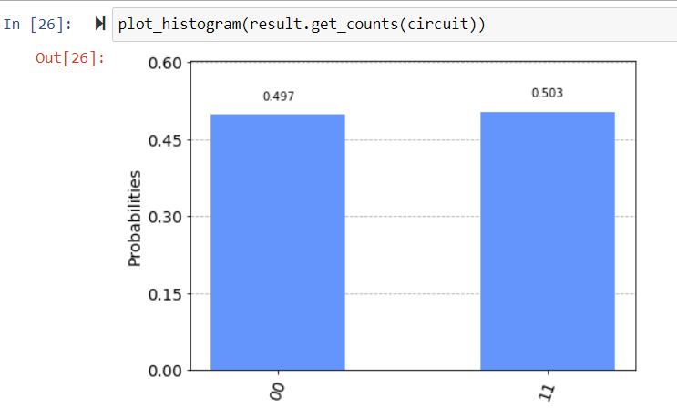
Now, we have the output of our circuit, which, makes sense as we have two possibilities, in a binary system, yields 50%, give or take error.
Next, we are going to load this program into one of IBM's supercomputers to determine if the results will be any different. This snippet is for loading our API token to call our account, which will allow us to use the actual quantum computer.
IBMQ.load_account()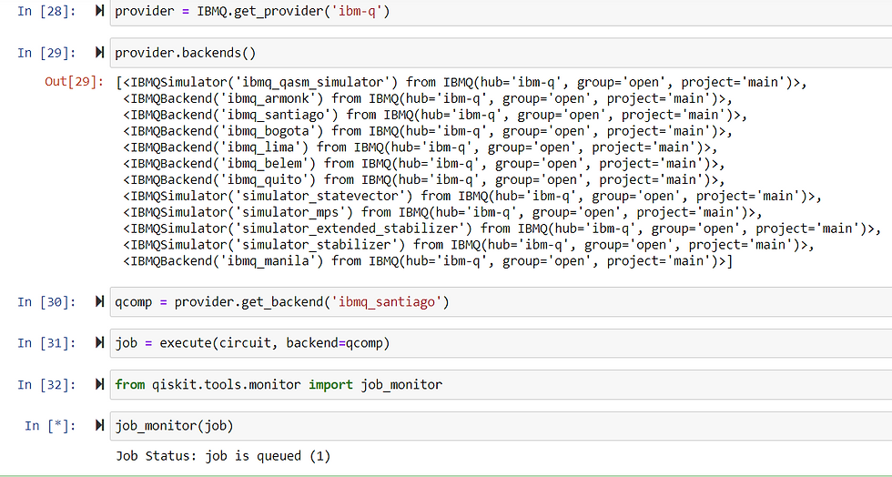
The job is queued and then subsequently will be run on the quantum backend we selected, we used 'santiago' from the list given by the command provider.backends().

Last but not least we will need to view our results again with the histogram function.
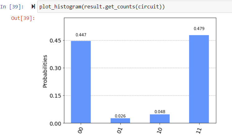
The difference between the two histograms is clear when our circuit is run on a real quantum computer, we get a few results in between the binary outcomes of the classical computer simulation.
Why does this happen? The simulator simulates a perfect quantum device, whereas the real quantum computer is susceptible to small errors. These errors are getting smaller and smaller every day as the technology developed becomes more accurate.
This was the simplest quantum program that could be run in Qiskit, I am eagerly looking forward to finding out what else I can do with Qiskit and how to contribute to the quantum computing community.


Comments